A Parametric CFD Model: Wind Turbine from Pipes

I’m building a wind turbine and as you might imagine, the blades are Ye Royale Paine In Me Buttocks. Too big for a CNC, too exposed for a 3D print, too complicated to be made by hand. I decided to make blades from pipes. This simplifies the build but now how do I know how to cut them?

I want to cut them so that they will produce as much torque in given wind conditions as possible. Now I know the question – the search for an answer may commence!

My Approach

There is a bunch of theory on blade aerodynamics but none of it covers my case. Since assumption is the mother of all f***ups, I decided to make none and just test a huge number of freely adjustable designs to find the best one.

Of course I have no intention to produce a huge number of simulations by hand. I’ll make virtual experiments with a CFD model and even those I will automate. The whole optimization process with be governed by an external tool. For the impatient, it’s called DAKOTA – but we’re not dealing with it just yet. First, we must prepare a black-box script that DAKOTA will run – the topic of this post.

The algorithm of choice will choose input parameters and pass them to a black-box script. It runs a simulation from given parameters. After it’s done, it passes results back to optimization program which in turn decides which parameters to pass to the next iteration. DAKOTA doesn’t give a wet slap about what’s going on in my script. I myself must prepare it so that it does the job.

The Black-Box Script

Here’s what it does:

1. Parses the parameters given by an external optimization program
2. Generates a CFD model of the geometry
   It is based on passed parameters and it changes every iteration.
3. Creates a mesh
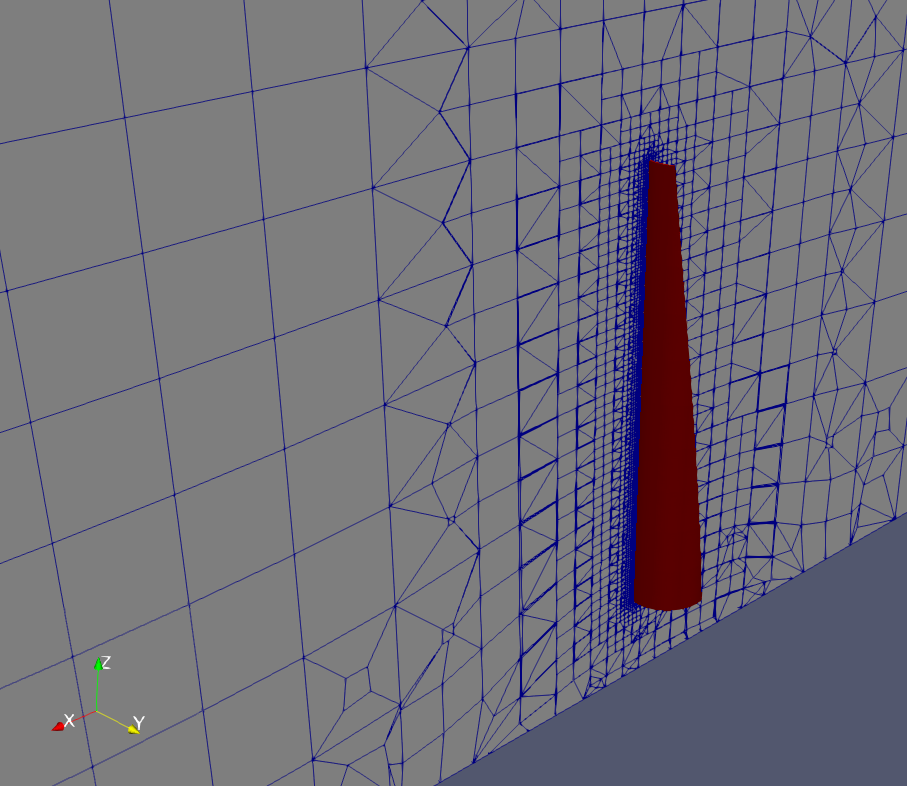
   That includes the air around a single blade and a lot of air up- and downstream of the rotor. I assume the other two blades behave the same – therefore I can copy them with a ‘cyclic’ boundary condition.
4. Sets up a CFD simulation
5. Runs the simulation
6. Post-processes the results
   In this case, we want to know what torque the blade produces . The script reads this value and returns it to the caller.

Geometry Definition

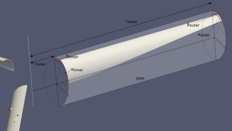
A blade’s geometry (how I decided to do it, anyway) is very simple. It is completely described by a few words – the following parameters:

• pipe diameter and wall thickness
• inner angle and span (βinner, αinner)
• outer angle and span (βouter, αouter)
• rotor inner and outer radius

If that’s not enough words for you to imagine, here’s a thousand more:

Inside an optimization iteration, we know these parameters. That means we can readily build the model.

CFD Model

With CFD we’re interested in what’s happening around our object. We don’t need a model of the object itself. We need a model of everything that object isn’t – its surrounding fluid.

A CFD model of a blade is simple and can easily be generated using blockMesh. But using that alonethe surrounding domain can’t possibly be created . This could heavily complicate the situation but fear not! I’ll still use blocks but with a plot twist from this blog post. Long story short, I’ll (ab)use blockMesh only to get the precious STL surfaces. snappyHexMesh will then come to the rescue.

To generate blockMeshDicts I’ll utilize my Grand Invention: classy_blocks.

classy_blocks: Blade

As I mentioned earlier, blade is made from a round pipe cut at the specified angles. This geometry is generated by several Loft operations between pre-calculated Faces. A Face is just a circular arc of specified thickness, starting at angle β and span angle α.

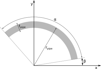
Creating such a face with classy_blocks is easy. Take two points on x-axis, namely (rinner, 0, 0) and (router, 0, 0). The face is defined by two pairs of these two points, first rotated by β, then by α. To generate a circular edge, another pair of points has to be specified: the same two initial points, rotated by (β+α)/2.

Put in code, a Face is generated like this:

import numpy as np
import parameters as p # (parameters parser)
from util import geometry as g
from operations.base import Face

def rot(point, angle):
    # rotates a 'point' by an 'angle' around z-axis
    return g.arbitrary_rotation(point, [0, 0, 1], angle, [0, 0, 0])

def circular_face(r, beta, arc):
    # creates a circular Face on specified 'r',
    # starting from angle 'beta' and spanning 'arc' angle 

    # r - radial location of the created face
    internal_vertex = np.array([p.pipe_diameter/2 - p.pipe_thickness, 0, r])
    external_vertex = np.array([p.pipe_diameter/2,                    0, r])

    inner_vertices = [
        rot(internal_vertex, beta),
        rot(internal_vertex, beta + arc),
        rot(external_vertex, beta + arc),
        rot(external_vertex, beta)
    ]

    # add a single point so that blockMesh will generate a circular edge
    inner_edges = [
        rot(internal_vertex, beta + arc/2), None,
        rot(external_vertex, beta + arc/2), None
    ]

    return Face(inner_vertices, inner_edges)

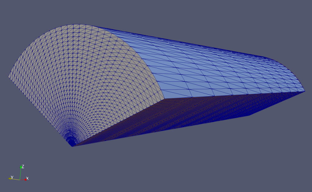
Note that blockMesh will treat all unspecified edges as straight lines. When cutting straight through a pipe at any angle (except axially) the result is always a curve. To obtain a geometry that would resemble a cut pipe, the simplest solution I could think of was simply to create a number of blocks from rinner to router. For each block a linear interpolation between βinner and βouter is used. The same goes for αinner and αouter.

from classes.mesh import Mesh
from operations.operations import Loft

# generate this many blocks span-wise;
# the higher the number, the smoother the curve
n_blocks = 10

mesh = Mesh()
betas = np.linspace(beta_inner, beta_outer, num=n_blocks+1)
arcs = np.linspace(arc_inner, arc_outer, num=n_blocks+1)
radii = np.linspace(p.r_inner, p.r_outer, num=n_blocks+1)

for i in range(n_blocks):
    inner_face = circular_face(radii[i], betas[i], arcs[i])
    outer_face = circular_face(radii[i+1], betas[i+1], arcs[i+1])

    block = Loft(outer_face, inner_face)
    block.count_to_size(0, p.pipe_thickness/2)
    block.set_cell_count(1, 1)
    block.set_cell_count(2, 10)

    mesh.add_operation(block)

classy_blocks: Domain

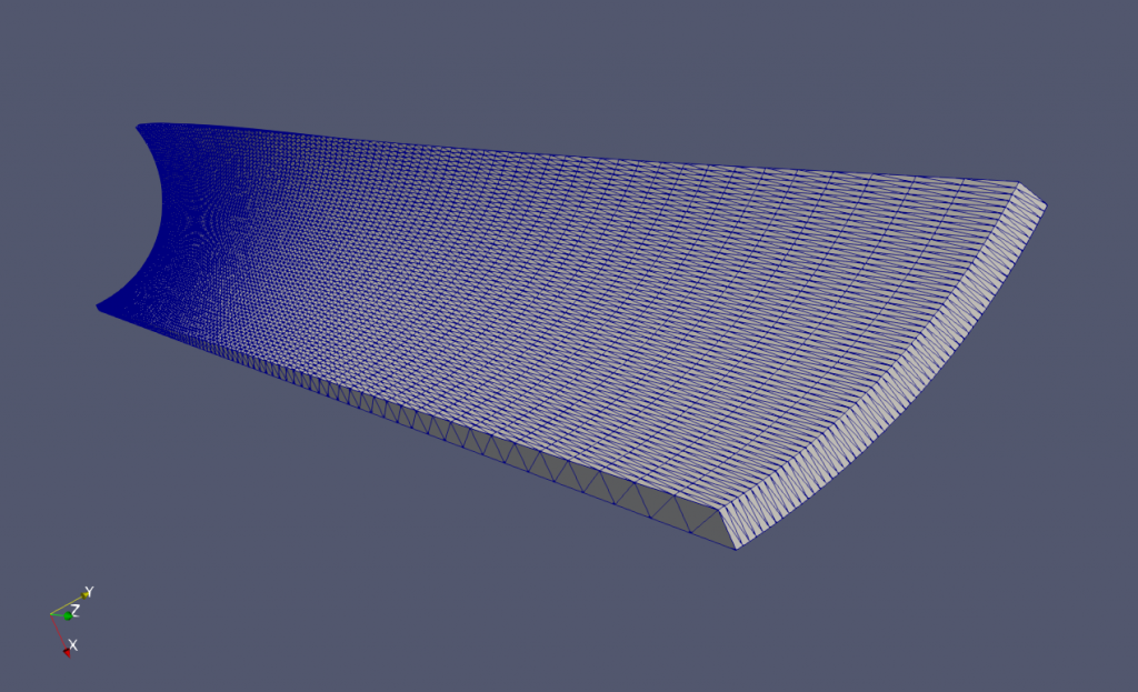
The domain is just a third of a cylinder. Could be Extruded from a circular-sector Face or a rectangle, revolved by 120°. I went for the latter. Most work actually went into specifying patches: cyclicLeft, cyclicRight, top, inlet, outlet. The bottom patch (block’s front side) is missing – it’s coincident with rotation axis.

from operations.operations import Revolve

# extension in the direction of flow (x-axis)
x_start = np.array([-3*p.r_outer, 0, 0])
x_end = np.array([5*p.r_outer, 0, 0])

# domain is a 120 degree section of a cylinder,
# revolved around y-axis
face = Face([
    x_start,
    x_end,
    p.outside_vertex + x_end,
    p.outside_vertex + x_start
]).rotate([1, 0, 0], -p.a/2)

domain = Revolve(face, p.a, [1, 0, 0], [0, 0, 0])
domain.set_cell_count(0, 10)
domain.set_cell_count(1, 30)
domain.set_cell_count(2, 30)

domain.set_patch('bottom', 'cyclicLeft')
domain.set_patch('top', 'cyclicRight')
domain.set_patch('back', 'top')
domain.set_patch('left', 'inlet')
domain.set_patch('right', 'outlet')

Case Organization

A directory in which everything happens includes the following:

• classy_blocks
  Cloned from github and with added parameters.py, generate_blade.py and generate_donut.py scripts.
• mesh
  This directory handles generation of three meshes:
  • blade geometry: system/blockMeshDict.blade
  • domain mesh: system/blockMeshDict.domain
  • background mesh for snappy: system/blockMeshDict.background
  • make_BMD.py: the script that actually generates background mesh for snappy. I talk about this very loudly in an ancient blog post about meshing shortcuts.
• case
  The actual simulation case. After the mesh has been finalized and polished, it is copied to constant/polyMesh in this directory. Here, only boundary conditions and whatnot is handled.
• Allrun script (see below).

Allrun Script

Allrun scripts from OpenFOAM tutorials are very simple but this one is a bit more complicated. Unfortunately with great complexity comes a great mess. Here’s an almost but not quite entirely non-messy script with all Bash (or my) awfulness included.

Let’s go slowly and with lots and lots of apologies.

#!/bin/bash
# parameters:
# (Here, the code that parses parameters from optimization program
# is omitted. It belongs to another blog post.)

# constants
r_inner=0.12 # [m]
r_outer=0.75 # [m]
pipe_diameter=0.125 # [m]
pipe_thickness=0.004 # [m]

# optimization parameters (fixed for now)
beta_inner=-120
arc_inner=120
beta_outer=-40
arc_outer=40

###
### CFD MODEL GENERATION
###
. $WM_PROJECT_DIR/bin/tools/RunFunctions
. $WM_PROJECT_DIR/bin/tools/CleanFunctions

### blade: create an STL file by extracting blockMesh patches
# blockMeshDict generation
cd classy_blocks

./generate_blade.py $r_inner $r_outer $pipe_diameter $pipe_thickness \
    $beta_inner $arc_inner $beta_outer $arc_outer
mv blockMeshDict.blade ../mesh/system/.

# blade surface extraction
cd ../mesh
cleanCase

runApplication -s blade blockMesh -dict system/blockMeshDict.blade
runApplication surfaceMeshExtract -constant constant/triSurface/blade.stl

If you compare generate_blade.py and generate_donut.py you will notice how many lines are dedicated to setting block patches in the latter but not a single is needed in the former. The whole blade is a single patch. Instead of juggling with block.set_patch() where first and last block need special treatment, I can just replace the defaultFaces region in STL file with blade. That is done with sed.

sed -i "s/defaultFaces/blade/" constant/triSurface/blade.stl

# domain surface, the same as blade
cd ../classy_blocks
./generate_donut.py $r_inner $r_outer $pipe_diameter $pipe_thickness \
    $beta_inner $arc_inner $beta_outer $arc_outer
mv blockMeshDict.donut ../mesh/system/blockMeshDict.domain

cd ../mesh
runApplication -s domain blockMesh -dict system/blockMeshDict.domain
surfaceMeshExtract -constant -patches "(inlet outlet cyclicLeft cyclicRight top)" constant/triSurface/domain.stl

###
### MESHING
###
# snappyHexMesh: create background mesh first

Warning, what comes next is something that escalated quickly. In a parametric CFD model, everything is related (scaled) with the parameters you chose. That involves multiplication, which Bash, amazingly, refuses to do (except with integers). I had two options, to use another cryptic utility (bc) or a slightly better known tool, Python.

#bg_mesh_size=$(bc <<< "scale=3;$pipe_diameter/1.1") # bc
bg_mesh_size=$(python3 -c "print(${pipe_diameter}/1.1)") # python

Passed and calculated parameters are then fed into make_BMD.py and inserted into dictionaries for topoSet.

./make_BMD.py constant/triSurface/domain.stl $bg_mesh_size
runApplication -s background blockMesh -dict system/blockMeshDict.background

# now everything is prepared to run: snappy and all
runApplication surfaceFeatureExtract
runApplication decomposePar -force
runParallel snappyHexMesh -overwrite
runParallel checkMesh -constant

# toposet: prepare topoSetDict to extract the right MRF zone
#mrf_radius=$(bc <<< "scale=3;$r_outer*1.2")
mrf_radius=$(python3 -c "print(${r_outer}*1.2)")

cp system/topoSetDict.template system/topoSetDict
sed -i "s/{{x1}}/-${pipe_diameter}/g" system/topoSetDict
sed -i "s/{{x2}}/${pipe_diameter}/g" system/topoSetDict
sed -i "s/{{radius}}/${mrf_radius}/g" system/topoSetDict

runParallel topoSet
runParallel setsToZones -noFlipMap

runApplication reconstructParMesh -constant

Then, and only, then, the mesh is complete. Moving on to ../case directory.

###
### SIMULATION
###
# prepare and run the case
cd ../case
cleanCase

# copy mesh from its directory
cp -r ../mesh/constant/polyMesh constant/
runApplication createPatch -overwrite
restore0Dir

# decompose and renumber
runApplication decomposePar -force -time 0
runParallel renumberMesh -overwrite
runParallel simpleFoam
runParallel -s postProcess simpleFoam -postProcess -func yPlus -latestTime

The simulation is done and results are ready: what’s left is to extract the relevant data – torque on the rotor. I would like to thank StackOverflow for kindly informing me about tail, tr, awk, cowsay and other useful tools.

# extract results from moment.dat
torque=$(tail -n 1 postProcessing/forces_blade/0/moment.dat | tr -d '()' | awk  '{print $2}')
cowsay "This design gives you a torque of $torque Mooton-meters"

At this point we have the $torque for this iteration. And that’s all! We can go outside and play now!

Well, not exactly. This what’s left to be done:

• Read parameters from an input file
• Write torque to output file
• Set-up DAKOTA and point it to this script
• Run a gazillion of iterations to find the best design.

But we’ll do this in another blog post.