OpenFOAM and DAKOTA: a Complete Guide

Running a single CFD simulation rarely provides enough information to find a good hydraulic or aerodynamic design of a component. In many cases the poor engineer has to wrestle an awfully long list of design parameters into a state-of-the-art shape. Luckily, OpenFOAM and DAKOTA together provide an almost ready-to-use solution just for that:

• Sensitivity analysis
  (long story short: checking which variable has the greatest influence on the result)
• Minimization
  (finding the optimum combinations of inputs for the best output)
• Model (curve, surface, …) fitting
• Uncertainty quantification
  (I have no idea what that is)
• And more
  (I also have no idea about all that)

This post is a guide to OpenFOAM and DAKOTA from installation to an optimized solution.

A Real-Life Solution

I’m building a wind turbine and right at the beginning my party was pooped by the most important element – the blades. I decided to cut them from pipes and scripted a program (called model from now on) that takes geometry parameters, runs a simulation and returns rotor torque. It’s rather complicated-ish so I dedicated a separate blog post to it. Have a look.

Once you have a model from which you can obtain results it’s just a matter of wrestling them into a combination that works best. Here, DAKOTA comes to help with its optimization talents. The recipe for working with it looks like this:

1. Specify input parameters for your model: ranges, values, names and whatnot.
2. Specify the model’s output – value we’re trying to minimize or maximize.
3. Point DAKOTA to your model (a script that does the calculation).
4. Choose which algorithm to use.
5. Run and wait. A long long time.
6. Check the results. The winning combination should be somewhere in the output files.

OpenFOAM and DAKOTA Installation

If you are reading this, you most probably already have OpenFOAM installed on your favorite platform. I’ll write instructions for installation of software I use because it’s not completely obvious and/or quirk-free. Even if no one needs that, I’ll have this guide as a note to self.

Windows: WSL2 and Ubuntu 20.04

If you’re using Ubuntu or any other Linux distribution, you don’t need this. But if you’re on Windows, installation procedures are well-documented: https://docs.microsoft.com/en-us/windows/wsl/install-win10

I really recommend WSL2 over the original WSL. The latter had some issues with disk I/O (my explanation) which caused apps to hang forever at totally random occasions. With WSL2, this problem seems to be gone.

I also recommend installing the latest Ubuntu version to WSL, that is 20.04 LTS at the time of writing. What’s great about it is that python3 is now default and python2 is nowhere to be seen. This really helps to reduce the confusion. (Not that it’s that important, though.) (Also not that it’s the only good thing about the latest Ubuntu.) (I actually don’t know what’s the difference between any of the versions.)

OpenFOAM

I use binaries for WSL, you can use whatever you prefer. The instructions on OF pages are just fine. Just stick to them.

Python: virtualenv

If you need to calculate pretty much anything, you’ll need numpy and scipy. Those two packages alone are quite heavy but you’ll probably need a few more. To keep them separated from other python things you and your system need, I highly recommend putting your calculation stuff in a virtual environment. I wouldn’t if it wasn’t so simple. For instance, I keep my wind-turbine-related environment in ~/venv/turbine:

sudo apt-get install python3-pip
sudo apt-get install python3-venv

python3 -m venv ~/venv/turbine

The environment has been created. To work in it, activate it with:

source ~/venv/turbine/bin/activate

You have to do this every time you open a new shell. If you want to deactive the environment to work on another one, just type deactivate.

Now, install whatever you need to do your magic:

pip3 install numpy scipy jinja2

With this setup, you should be ready to run a single iteration from this post.

DAKOTA

The guys at Sandia are a little stingy with binaries – they only provide one for Linux, and that is for Red Had Enterprise, which is something I do not have. So you have to compile it from source. It takes a while but with these instructions hopefully you’ll make it.

First, prerequisites: stuff you need for compilation.

sudo apt-get install gcc g++ gfortran cmake libboost1.67-all-dev libblas-dev liblapack-dev libopenmpi-dev openmpi-bin gsl-bin libgsl-dev python perl libhdf5-dev cowsay

Then, create a directory to hold source and binaries. To keep things simple, chown it:

cd /opt/
sudo mkdir dakota
sudo chown $USER dakota
cd dakota

You’ll also need the source. Download it from this page. If it’s a bit confusing – select Source (Unix/OS X), then Release 6.12, Command Line Only, Supported. When download finishes, move it to this directory and unzip it:

cp /mnt/c/Users/<user>/Downloads/dakota-6.12-release-public.src.tar.gz .
tar -xvzf dakota-6.12-release-public.src.tar.gz
rm dakota-6.12-release-public.src.tar.gz

Now you’re ready for compilation. Make a build directory, configure and compile. We’ll stick to defaults so there’s no need for all complications in the official instructions.

Don’t forget to change the number of processors for make command. For a bonus little stress-test of your computer.

mkdir dakota-build
cd dakota-build
cmake ../dakota-6.12.0.src/
make -j <1.5x number of your physical cores>
# This might take a while... Stay strong!
make install .

Hopefully everything went OK. If it did, you can run DAKOTA:

cd ~
nejc@Buquica:~$ dakota --version
Dakota version 6.12 released May 15 2020.
Repository revision 35a9d0d5b (2020-05-13) built Oct 15 2020 22:12:47.

Voilá!

Installation and Compilation Caveats

libboost-all-dev breaks something with version 1.71 so it throws an error boost_find_component Macro invoked with incorrect arguments for macro. The newest previous available version for Ubuntu 20 at the time is 1.67 – so we install that.

The last step of OpenFOAM installation requires you to add a source command to .bashrc (source /opt/OpenFOAM/OpenFOAM-v2006/etc/bashrc). This now forces other programs to use OpenFOAM’s libraries which makes them very miserable (dakota is among them):

dakota: /opt/OpenFOAM/ThirdParty-v2006/platforms/linux64/gcc-6.3.0/lib64/libstdc++.so.6: version `GLIBCXX_3.4.26' not found (required by /usr/local/bin/../lib/libteuchosparser.so.12)

I did not go too deep into research why this happens – all my problems were solved by adding another line to ~/.bashrc:

export LD_PRELOAD="/usr/lib/x86_64-linux-gnu/libstdc++.so.6"

Restart the shell and both OpenFOAM and DAKOTA should now coexist peacefully:

simpleFoam --help
dakota --version

OpenFOAM and DAKOTA: Workflow

Model

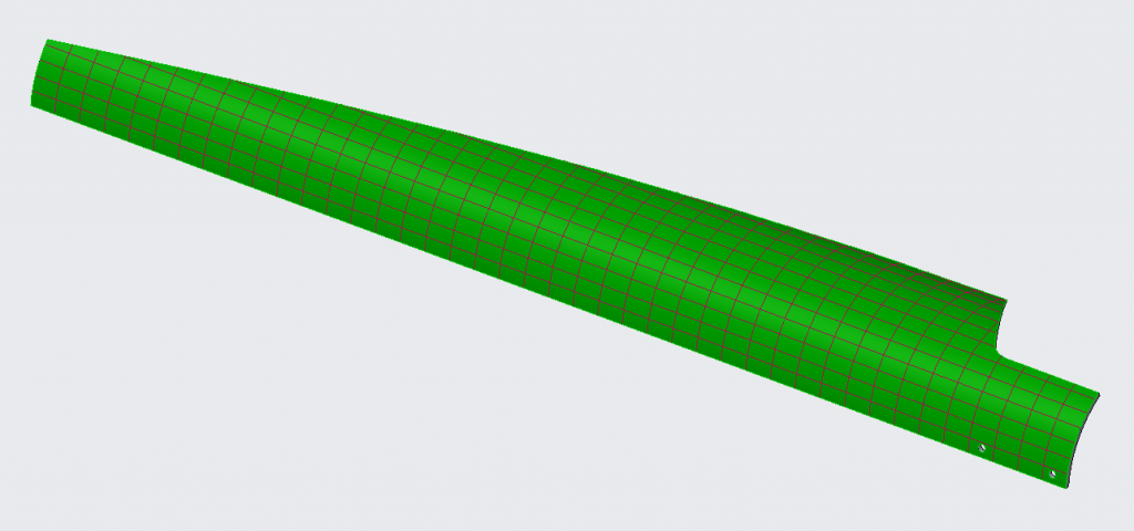
Just to remind you: we’re shaping a wind turbine blade cut from a pipe. We’re searching for the best combination of parameters – the one that will give the highest torque output.

This is a black-box script from another post. It takes four parameters: inlet angle and (angular) blade span at root and tip of the blade. Other four parameters are fixed – I chose turbine diameter and available pipe dimensions in advance. I just want to know how to cut it.

 ___________________________________
/ This design gives you a torque of \
\ 0.005918680e-03 Mooton-meters     /
 -----------------------------------
        \   ^__^
         \  (oo)\_______
            (__)\       )\/\
                ||----w |
                ||     ||

The Algorithm

We’ll be dealing with a single chapter among DAKOTA’s capabilities: optimization. There’s no point in explaining this stuff because it’s already much-too-well explained elsewhere. Our algorithm must meet a few criteria:

1. multiple input parameters
   (4 in this case)
2. no gradients
   (the simulation can calculate a single point and that’s it)
3. noisy data
   (resulting function will not be microscopically smooth)
4. concurrent evaluations
   (that isn’t critical but it would be nice to work on multiple points at once)

Almost anything can manage #1 and #2. But! #3 and #4 are bad news. Anyhow, some can do all of the above so I chose the dividing rectangles method. It proved quick and robust not only in this case but also in optimization sessions with 7 variables and more.

Input file

Before I bury you with tons of configuration text, let’s sum up what I want OpenFOAM and DAKOTA to do for me:

• Find a combination of 4 blade parameters
  • that give the maximum torque,
  • using a dividing rectangles method,
  • stopping at a certain tolerance,
  • limiting input values to physically manufacturable shapes.
• Provide additional 4 parameters
  • that don’t change between iterations.
• Obtain blade torque from each iteration
  • by running my custom black-box model
  • which cannot provide information about gradients or hessians or whatever.
• Write all results to a text file.

That’s it. All that is left to do is to translate the above list to whatever DAKOTA will understand. The blade.in file explains itself:

environment
    # write results to this file
    tabular_data
        tabular_data_file = 'results.dat'

method
    # use the dividing rectangles method;
    coliny_direct
    # and don't optimize beyond precision
    # our model can provide
    min_boxsize_limit = 0.2

variables
    # specify our 'design' variables - parameters
    active design
    continuous_design = 4
        descriptors     'beta_inner'  'arc_inner'  'beta_outer' 'arc_outer'
        lower_bounds           -180           30          -180          20
        upper_bounds            180          175           180          95
        # initial point is optional for dividing rectangles
        # (see chapter mapFields)
        initial_point           -90           90           -90          90

    # these parameters will be included in the input file but will remain
    # fixed with these values
    continuous_state = 4
        descriptors     'r_inner' 'r_outer' 'pipe_diameter' 'pipe_thickness'
        initial_state       0.12      0.75           0.125            0.004

interface
    fork
        # dakota will 'fork' this script for each iteration;
        # two command-line parameters will be appended,
        # input file path (iteration parameters)
        # and output file path (results)
        analysis_driver = 'run'

responses
    # at the end of each iteration, DAKOTA will
    # read the output file and look for a variable named 'torque'
    objective_functions = 1
    descriptors 'torque'

    # what our model can't provide
    no_gradients
    no_hessians

    # we're not minimizing but maximizing
    # our function
    sense 'max'

Parsing and Passing Parameters

By default dakota will create an input file somewhere in /tmp/ directory and pass its path as the first argument to our run script. The file will contain all variables that we need but in a totally useless format. Fortunately guys at Sandia figured that out themselves and provided a preprocessing script that creates a more pleasant format. We can write a template file where we specify the input format. If we write it correctly, we can store the contents of the file directly into variables – which are then available throughout the run script as $r_inner, $r_outer, etc.

dprepro $parameters_file parameters.template parameters.in
# the parameters.template is written in a way it can be read directly:
. parameters.in

At this point our scripts are ready to run but there’s one more detail I’d like to clarify before your computer catches fire.

mapFields

Since we will be running dozens of iterations with very similar geometry, we can speed up the convergence by initializing our fields from previous iterations.

The first iteration will start un-initialized and wil therefore need a little longer to converge. It will save the results to a separate case which will then be used by all other iterations. They will start from a better initial internalField and converge much, much quicker.

The first iteration will know it’s the first by reading results.dat file that dakota writes to live.

iteration_no=`wc -l < results.dat`

if [[ $iteration_no == "1" ]]; then
    # first iteration: initialize fields with potentialFoam
    runParallel potentialFoam
else
    # all next iterations: map fields from 'initial'
    runApplication mapFields -consistent -parallelSource -parallelTarget -mapMethod mapNearest -sourceTime latestTime ../initialized
fi

#runParallel simpleFoam
#...

After the first iteration is done, it saves the case directory to initialized for the successors.

cd ..
if [[ $iteration_no == "1" ]]; then
    rm -r case_zero
    cp -r "case" case_zero
fi

Run!

Now we call dakota and provide the above file as input with an -i blade.in option. If you don’t want it to throw the output text up all over your terminal, provide an -o output.log option:

dakota -i blade.in -o output.log

Now wait for the results. A long long time.

The Results

If everything went OK, results.dat file we specified in blade.in will contain parameters and outputs from all iterations. At the end of output.log you can find which iteration was the best. You’ll have all the parameters if you open the results.dat file and look for the mentioned iteration.

%eval_id interface     beta_inner      arc_inner     beta_outer      arc_outer        r_inner        r_outer  pipe_diameter pipe_thickness         torque 
1            NO_ID              0          102.5              0           57.5           0.12           0.75          0.125          0.004  -0.0832453759 
2            NO_ID            120          102.5              0           57.5           0.12           0.75          0.125          0.004  -0.0842540585 
3            NO_ID           -120          102.5              0           57.5           0.12           0.75          0.125          0.004   0.0175737057 
...
...
...

Now it’s time to stop crunching numbers and start drawing!

A Few More Hints

Concurrent Iterations

If you have a sick number of cores available or if your domain is stupidly small (read: 2D), instead of over-decomposing it might be a better idea to run multiple iterations at once, each with a single core (or very little of them). evaluation_concurrency is the keyword here. Keep in mind that how many you can run is also determined by the algorithm and number of free variables. Here’s what the docs say about dividing rectangles: “The DIRECT algorithm supports concurrency up to twice the number of variables being optimized.“

In this case you will need to isolate iterations by putting them in separate directories. See the description of work_directory keyword. Most probably you’ll also need some config files/scripts to work with: see link_files and copy_files commands.

Keeping Iteration Results

DAKOTA will happily wipe finished iterations’ files. If for whatever (debugging) reason you want to keep them, use file_save (input/output files) and directory_save.

Input and Output Filter

In this tutorial we wrote a single script that handles everything. Geometry calculations, model generation, simulation set-up and postprocessing. For a more complex model it might be convenient to have separate scripts. For instance, a python script for calculations and configuration, an Allrun shell script and another python script for postprocessing calculations. That’s why dakota offers input_filter, analysis_driver and output_filter keywords. Even more, you can specify multiple scripts to be run for every command.

Reset and Failure

If your optimization session is stopped for any reason you can continue from the last successful step. By default DAKOTA creates a dakota.rst file. If dakota -i blade.in -read_restart dakota.rst it will try to continue where it left off.

When an iteration crashes/fails/doesn’t return a result, DAKOTA will lose it and refuse to continue. Here’s how you handle that:

1. Set failure_capture keyword.
2. Decide how to handle failures: for my cases, recover was the best option.
3. Decide which number to use on fail. For instance, when optimizing efficiency, a 0 might be in order. When looking for a greatest torque, a sufficiently negative number will do.
4. The first thing your scripts do should is to write a results file. The contents: fail. (case-insensitive)
5. If the iteration succeeds, rewrite the results file with… results.
6. If the iteration fails, the fail string will tell DAKOTA something went wrong and it wil use the number from #3 as result.

Multiple Objectives

DAKOTA can optimize functions that return many values. It does that by combining outputs with weights the user specifies. I have no experience with multiobjective optimization. Anyway, you might still want your model to return multiple values (for instance, lift and drag, weight, efficiency, whatever). In this case you can specify multiple response_functions. Then you assign weights of 0 to every response except the one you’re optimizing.

Don’t forget to update failure_capture > recover with a separate value for each response.

A More Proper Configuration

Here are all of the above hints translated to DAKOTAian. Just so you know where to put all the stuff.

interface
    asynchronous
        evaluation_concurrency = 8

    fork
        analysis_driver = 'Allrun'
            input_filter = '/opt/blade/prepare.py'
            output_filter = '/opt/blade/postprocess.py'


        work_directory
            copy_files '/opt/blade/case'
            named 'dakota_work/iteration'

            directory_tag
            directory_save

        file_tag
        file_save
        
    failure_capture
        recover -100 0 0 100

responses
    objective_functions = 3
        descriptors 'torque' 'lift' 'drag' 'mass'
        weights           1      0      0      0
    
    no_hessians
    no_gradients

    sense 'max'

OpenFOAM and DAKOTA Files

Here’s the whole blade optimization thing without results. It should work on a setup described above.

Have fun and good luck!