classy_blocks Tutorial Part 7: Optimization

This is the 7th part of the classy_blocks tutorial. It is highly recommended that you read part 6 because we’ll use curves and whatnot.

Mesh Quality

The Finite Volume Method (FVM) not only requires discretization of geometry into simpler basic elements (called cells) but is also terribly picky about their shape. It can work with anything from a tetrahedron to an arbitrary polyhedron. Nevertheless, hexahedral meshes, aligned with the flow, have proven to be the best for most CFD needs. Alas, this is not the only requirement. FVM wants those cells to be as pretty as possible. How pretty is defined by a rather large number of mesh quality criteria – I will not repeat everything here but I do highly recommend the above two excellent Wolf Dynamics presentation (and indeed, their other stuff too!). Those criteria seem to be the most important – check them out:

• Non-orthogonality
• Skewness
• Aspect ratio

I have added a fourth one, inner angle. This is simply an angle between two cell faces, sharing the same edge. Improving inner angles will lead to better skewness and non-orthogonality which will be beneficial to our optimization process.

The classy_blocks Approach

The idea is simple:

• Define your blocking with a simple sketch
• Place blocks approximately
• Decide which block vertices can be moved, how much and in which direction
• Move the above vertices around until the best possible block quality is obtained
• Add all other data (cell counts and gradings, patches, curved edges, etc.)
• Write the optimized mesh.

You should already know the first two and the last two pretty well. I’ll explain about the rest in this tutorial.

Block Quality

There is no such thing as block quality. In block-structured meshes, blocks are chopped into hexahedrons and only then each cell is checked for quality.

However, we have no idea what shape our cells will be before we even place our blocks! So we can treat each block as a single huge hexahedral cell and calculate its quality using the same equations as for a single cell. If it shows good promise there is a good chance cells will also be fine (see below) but if it’s bad there is no way chopped cells will be fine.

Multiple Criterions

Optimizing a function that returns a scalar is straightforward. On the contrary, multiobjective optimization is a difficult business. Instead wrestling with that, classy_blocks sums up all criteria and then optimizes them all at once.

However, one can not sum up two numbers with different units or meaning. Before summing, each quantity is transformed with a special function. That function is tuned so that it yields small values for okay-ish qualities but as each criterion approaches unacceptable values its value increases exponentially. That ensures optimizer works on worst parts of the mesh and does not spoil good ones in the process.

Limitations

Curved Edges

Since we treat blocks as a single cell, we cannot take curved edges into account. Although theoretically possible, this has not yet been implemented into classy_blocks. You will see – already in this tutorial – where this might be a problem but you will also see how this is not really a problem in a properly defined case.

2D geometry

Two-dimensional meshes have a fixed thickness in 3rd dimension, that is, 1 unit. If your object is very small (orders of magnitude less than 1), cells will have huge aspect ratio (ratio of longest to shortest edge length). Optimization algorithms will see those cells as being very bad because of this but solvers will ignore this.

Cell Quality

This one is the most obvious – we have no idea about cell quality until we actually make them. Curved edges will produce high non-orthogonality and skewness, thin cells at boundary layer will have high aspect ratio, projected entities might ruin everything very quickly, etc…

Luckily most of these problems can be avoided by having a good blocking scheme. Also, experience helps.

Now let’s get our hands dirty.

An Example: Airfoil Generator

We want to analyze a NACA 2414 airfoil at different angle of attacks (AoA). We have a .dat file with a set of 2D points describing the profile at zero AoA. Now we need a mesh so we can make some pretty pictures.

Geometry Setup

NACA airfoils have blunt trailing edges. Some engineers sharpen them to zero thickness but we’ll take advantage of this and use a blocking scheme where thin and long cells near airfoil do not propagate into wider domain.

Keep in mind I am not an expert on airfoils and dynamics thereof so I don’t know what damage I have done by doing that. But I know that aeroplane wings are not razor-sharp at ends because that would make life of airport personnel much more miserable.

This is our blocking:

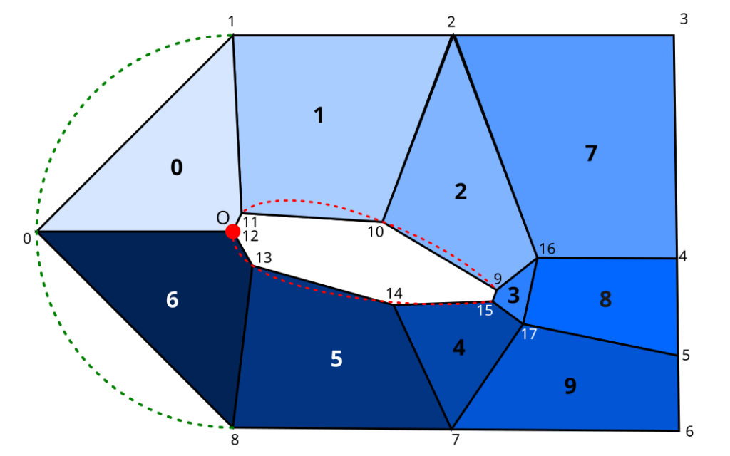
Small numbers denote points, bold numbers are block indexes. Red line is our imported NACA curve, green arc is a future inlet edge of our domain. Red point O denotes coordinate system origin (and is not necessarily coincident with any of the other points.

Construction

The following recipe is my way of creating 2D or rotational geometries and is not enforced by classy_blocks. I will include it because I guess it’s handy and it will also make other parts of tutorial more clear.

First, we need two curves, one for the bottom of the mesh and one exactly the same but on the top. We covered that in detail in the previous tutorial so let’s just say we have these two Curve objects:

foil_curve = get_curve(0)
top_foil_curve = get_curve(1)

They are already scaled to CHORD and rotated to ANGLE_OF_ATTACK in the get_curve() function. thickness is a vector (0, 0, 1), used as a shortcut throughout the script.

Points

We’ll place our points approximately by some rough estimates, based on CHORD:

points = np.zeros((18, 3))
points[0] = [-CHORD / 2, 0, 0]
points[1] = [0, CHORD / 2, 0]
points[2] = [CHORD, CHORD / 2, 0]
points[3] = [1.5 * CHORD, CHORD / 2, 0]
points[4] = [1.5 * CHORD, CHORD / 4, 0]
points[5] = [1.5 * CHORD, -CHORD / 4, 0]
points[6] = [1.5 * CHORD, -CHORD / 2, 0]
points[7] = [CHORD, -CHORD / 2, 0]
points[8] = [0, -CHORD / 2, 0]

We obtain points 9 to 15 from the bottom curve.

for i, point in enumerate(foil_curve.discretize(count=7)):
    points[i + 9] = point

We’ll update point 12 so that it is the one closest to point 0. This is to provide the best starting point for later optimization business.

points[12] = foil_curve.get_point(foil_curve.get_closest_param(points[0]))

Points 16 and 17 are not placed on any specific entity so let’s just take averages from their neighbours. It’ll be okay for a start:

points[16] = np.average(np.take(points, (9, 4, 3, 2), axis=0), axis=0)
points[17] = np.average(np.take(points, (15, 5, 6, 7), axis=0), axis=0)

Lofts

We have the points, now let’s write down the faces they will define:

loft_indexes = [
    [12, 11, 1, 0],  # 0
    [11, 10, 2, 1],  # 1
    [10, 9, 16, 2],  # 2
    [9, 15, 17, 16],  # 3
    [15, 14, 7, 17],  # 4
    [14, 13, 8, 7],  # 5
    [13, 12, 0, 8],  # 6
    [2, 16, 4, 3],  # 7
    [16, 17, 5, 4],  # 8
    [17, 7, 6, 5],  # 9
]

Each entry in this list defines a Face. We copy that and translate by thickness and voila, we have our lofts ready!

def get_loft(indexes):
    bottom_face = cb.Face(np.take(points, indexes, axis=0))
    top_face = bottom_face.copy().translate(thickness)

    loft = cb.Loft(bottom_face, top_face)
    loft.set_patch(["top", "bottom"], "topAndBottom")

    return loft

lofts = [get_loft(quad) for quad in loft_indexes]

Edges

We have blocks that have front faces on the airfoil curve, we have the curves. Specifying edges is now as easy as it gets:

for i in (0, 1, 2, 4, 5, 6):
    loft = lofts[i]
    loft.bottom_face.add_edge(0, cb.OnCurve(foil_curve))
    loft.top_face.add_edge(0, cb.OnCurve(top_foil_curve))

We should not forget the round inlet:

for i in (0, 6):
    lofts[i].bottom_face.add_edge(2, cb.Origin([0, 0, 0]))
    lofts[i].top_face.add_edge(2, cb.Origin(thickness))

Now we only need to chop those lofts and add them to the mesh and we are able to write it down. I’ll skip those parts because they are not relevant.

Now we assemble our mesh:

mesh.assemble()

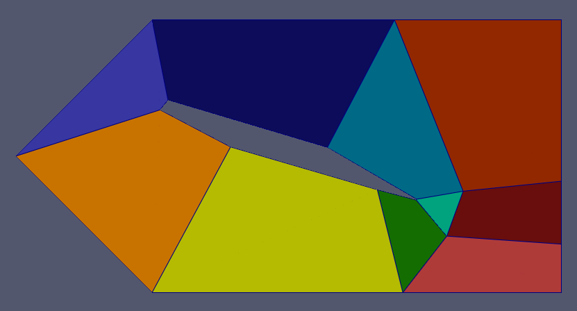
Here is our blocking:

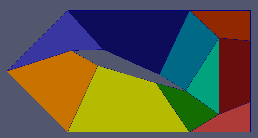
Block 0 is concave and cells within it would cause any solver to crash immediately. However, after adding curved edges and chopping them, it actually isn’t that bad. Alas, this is not the case for blocks 3 and 9.

You can immediately spot areas with bad cells. checkMesh is also not very happy:

    Mesh non-orthogonality Max: 84.7714 average: 32.5949
   *Number of severely non-orthogonal (> 70 degrees) faces: 231.
    Non-orthogonality check OK.
  <<Writing 231 non-orthogonal faces to set nonOrthoFaces
    Face pyramids OK.
 ***Max skewness = 7.64087, 5 highly skew faces detected which may impair the quality of the results
  <<Writing 5 skew faces to set skewFaces
    Coupled point location match (average 0) OK.

Failed 1 mesh checks.

Clamps

If we fiddled manually with the points list we would definitely be able to provide better defaults and thus a better mesh. But the moment we rotate the airfoil to a different AoA, this will all fall apart. So let’s automate this. We’ll move the points like this:

• 10, 11, 12, 13, 14: along the airfoil curve where they have already been placed. Point 12 has already been nicely placed and points 9 and 15 must be fixed on the trailing edge.
• 16, 17: move freely on x-y plane.
• 2 and 7: horizontally only
• 4 and 5: vertically only

Point 0 remains fixed.

Mind that points that we defined and are in use by Lofts (and other operations) are not the same as vertices, created when we assembled the mesh. Lofts keep their own points whereas Vertices are shared among all blocks that were built from operations. Therefore we have to find Vertices from points. classy_blocks provide different finders, in this case (where we know the exact location of the points) a simple GeometricFinder will suffice. We’ll define a helper function that will fetch the first (and the only) vertex at point from our list:

finder = cb.GeometricFinder(mesh)
optimizer = cb.Optimizer(mesh)

def find_vertex(index):
    return list(finder.find_in_sphere(points[index]))[0]

Clamps are objects that define where a specified Vertex can go during optimization and where it can’t. Let’s create them and feed them to the optimizer.

Curve

We already have our Curve, just feed it to CurveClamp.

for index in (10, 11, 13, 14):
    opt_vertex = find_vertex(index)
    clamp = cb.CurveClamp(opt_vertex, foil_curve)

    optimizer.release_vertex(clamp)

Plane

A Plane is defined by a point and normal. In this case it is as simple as it gets:

for index in (16, 17):
    opt_vertex = find_vertex(index)
    clamp = cb.PlaneClamp(opt_vertex, [0, 0, 0], [0, 0, 1])

    optimizer.release_vertex(clamp)

Line

We’ll take a little shortcut here as well:

def optimize_along_line(point_index, line_index_1, line_index_2):
    opt_vertex = find_vertex(point_index)
    clamp = cb.LineClamp(opt_vertex, points[line_index_1], points[line_index_2])

    optimizer.release_vertex(clamp)

optimize_along_line(2, 1, 3)
optimize_along_line(7, 8, 6)
optimize_along_line(4, 3, 6)
optimize_along_line(5, 3, 6)

Links

Optimizer now has enough data to improve our blocking. Except that it won’t do a good job because all clamps refer to points on bottom plane. We have completely omitted top points. We could add them to optimization as well. But this would double our degrees of freedom, and because optimization is not terribly accurate (it doesn’t need to be), the optimized mesh would not be 2D anymore.

What we do instead, is add links. A Link is an object that connects two Vertices: a leader and a follower. The first is also passed to a Clamp and its position is modified during optimization. The second merely keeps the same distance between them.

In this case we add a TranslationLink to each Clamp but if we were building a 3D mesh of some kind of round geometry, a RotationLink is also available.

def make_link(leader):
    # Find the respective point in the top plane and
    # create a link so that it will follow when
    # leader's position changes
    follower_position = leader.position + thickness
    follower = list(finder.find_in_sphere(follower_position))[0]

    return cb.TranslationLink(leader, follower)

# for each clamp:
clamp.add_link(make_link(opt_vertex))

Optimization Algorithm

Let’s run the optimizer:

optimizer.optimize(tolerance=1e-5)

You’ll see output like this:

Starting iteration 1 (relaxation 0.50)
  > Optimized junction at vertex 17: 1.761e+04 > 1.676e+04
  > Optimized junction at vertex 13: 1.676e+04 > 1.522e+04
  > Optimized junction at vertex 1: 1.522e+04 > 1.348e+04
  > Optimized junction at vertex 21: 1.348e+04 > 1.341e+04
  > Optimized junction at vertex 32: 1.341e+04 > 1.325e+04
  > Optimized junction at vertex 20: 1.325e+04 > 1.292e+04
  > Optimized junction at vertex 8: 1.292e+04 > 1.292e+04
  > Optimized junction at vertex 9: 1.292e+04 > 1.288e+04
  > Optimized junction at vertex 28: 1.288e+04 > 1.226e+04
  > Optimized junction at vertex 24: 1.226e+04 > 1.226e+04
Iteration 1 finished. Improvement: 1.761e+04 > 1.226e+04

Here’s what’s going on:

• Optimizer creates Junctions from Clamped vertices and calculates quality of all blocks that each vertex defines.
• It finds the worst junction and tries to move the vertex so that quality of the blocks it defines is improved.
• If it doesn’t succeed, it will rollback to original position.
• When all junctions have been optimized, it will return back to the first one and repeat the procedure.
• The algorithm stops when improvement in the last iteration is less than tolerance fraction of the first improvement (not original quality!) or iteration limit is hit (max_iterations).

Relaxation that is mentioned within report is similar to under-relaxation in CFD solvers. It will limit point movement in the first iterations. This will minimize problems where extremely bad blocks would be improved on account of their neighbours – they could be ruined at the same time.

You’ll have to play with tolerance a bit. Depending on the case, something like 0.1 could be sufficient but in this, airfoil case, 1e-5 or even 1e-6 only starts to produce good results.

Results

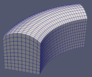
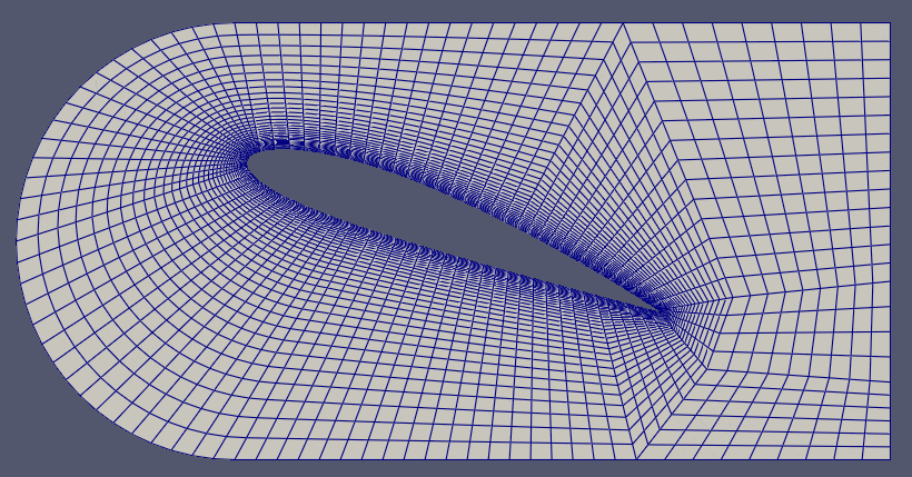
This is the optimized blocking:

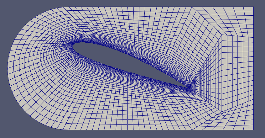
And the mesh:

checkMesh is now happy:

    Max aspect ratio = 32.3009 OK.
    Minimum face area = 1.13019e-07. Maximum face area = 0.0339744.  Face area magnitudes OK.
    Min volume = 1.13019e-07. Max volume = 0.000749401.  Total volume = 0.449048.  Cell volumes OK.
    Mesh non-orthogonality Max: 52.8421 average: 15.7103
    Non-orthogonality check OK.
    Face pyramids OK.
    Max skewness = 1.22312 OK.
    Coupled point location match (average 0) OK.

Mesh OK.

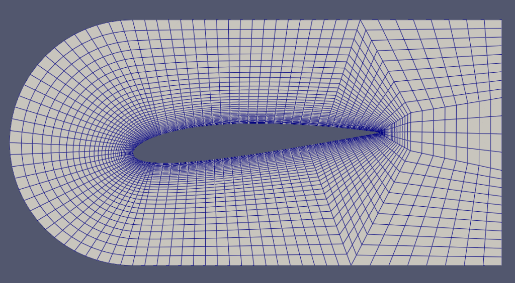
A different AoA

Let’s do the same for a different AoA all over again. Except that we don’t need to anything except change one number and wait for the optimizer to do its job:

Conclusion

In this classy_blocks tutorial, we used roughly 150 lines to create a fully-functional parametric airfoil mesh generator. Of course, for proper usage one would have to add another layer of blocks to extend the domain (a single Shell shape on left, top and bottom side, then an Extrude on each of the 5 faces on the right). There is still some work to do on chopping (cell size transition between blocks) and probably some testing at different AoA and with different airfoils.

At the moment the Optimizer is terribly slow so try to keep number of degrees of freedom (a.k.a. Clamps) as low as possible.

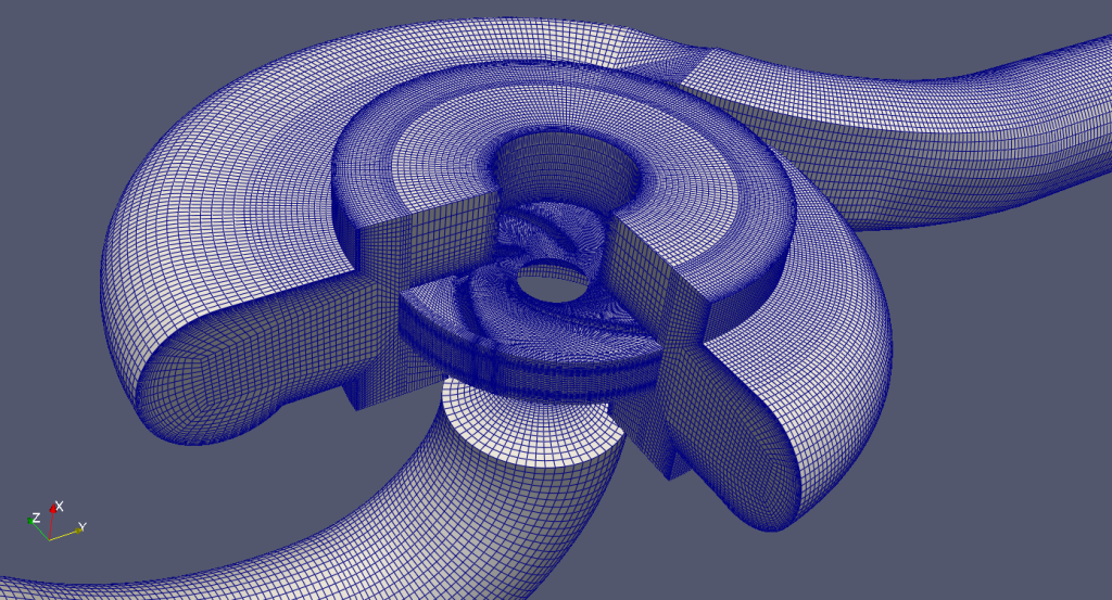
Also, this is not the only thing Optimizer can do – for instance, this pump mesh is made only with blockMesh. Optimizer is used for blocks on suction pipe/impeller inlet, impeller channel and volute spiral. It takes a while to obtain a mesh like that but it is well worth it. The results are much, much better than any other open source automatic mesher and that with much lower cell count!

Compared to the above, this airfoil generator is a relatively simple script. But things get complicated very quickly and a single file becomes messy and unmanageable. In that case I’d recommend splitting it into objects and dataclasses that take case of assets like Points and Curves, then maybe Sketches that create faces from whatever assets, then maybe Clamp collectors for optimization, and so on. A properly organized meshing script will create meshes you never knew you could make!

Until next time… happy meshing!