This is the 5th part of the classy_blocks tutorial. Its contents are rather advanced-ish so before you dive into it you should really know the basics first.
This article is a preparation chapter for the next sort-of-serious tutorial, optimization.
But First, a Pep Talk
(Which you can easily skip if you’re motivated enough already)
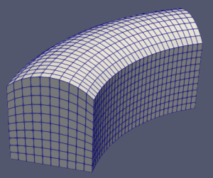
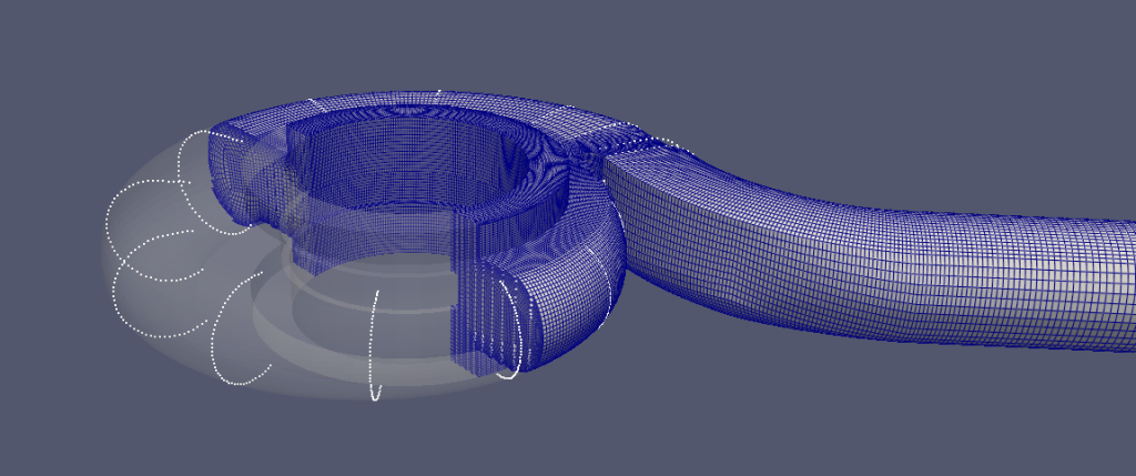
Alas, we do not live in Minecraft so there are some objects of interest that are curved. More specifically, turbomachinery (impellers, propellers, volutes, blades of any kind), all sorts of aerodynamic shapes, airfoils, piping, organic shapes (blood vessels), peristaltic pumps, and the list goes on and on.
Often these shapes are developed or at least described by a series of cross-section curves, or their edges are curved, or both, or something completely different. Experience shows that working with a rudimentary Spline edge gets clumsy and tedious and the solution comes with classy_blocks 1.3.3: the Curve objects.
classy_blocks Curves
A curve is a function that takes a single parameter (say, $t$) and returns a point in 3D space:
$$P(x, y, z) = f(t)$$
It is defined on a certain interval $t_1 <= t <= t_2$ (or at least clipped to it). classy_blocks currently provides the following tools:
- get a point on this curve by providing parameter $t$
- calculate length of curve within specified bounds
- find a parameter that yields a point on curve that is the closest to an arbitrary point
- discretize the curve into $n$ points between speficied bounds
- transform – translation, rotation, scaling (but not all kinds of curves, see below)
Other methods or properties are not yet implemented but can be done easily:
- tangent vector
- normal vector
- curvature
- extrapolation beyond bounds
- …
You can quickly add your own if you subclass your chosen classy_blocks curve.
Analytic Curve
A circle in x-y plane would be defined as:
$$P(x, y, z) = (\cos 2 \pi t, \sin 2 \pi t, 0)$$
This is an analytic curve, parameter t goes from $0$ to $1 \pi$ and it completely describes everything that’s going on.
To define an analytic curve for classy_blocks, you need that function and bounds within which to stick. Alas, transforming analytic curves is not supported because poor Python has no mathematical knowledge about the provided function.
For example let’s construct a circle and see if its length is what it’s supposed to be:
>>>import classy_blocks as cb
>>>import numpy as np
>>> circle_curve = cb.AnalyticCurve(lambda t: np.array([np.cos(2*np.pi*t), np.sin(2*np.pi*t), 0]), (0, 1))
>>> circle_curve.length
6.2831853094400785
>>> 2*np.pi
6.283185307179586
Constructing a circle like that obviously works but a few excursions like that and your brain is fried for the day. Therefore classy_blocks nicely provides shortcuts to preserve brain for better jobs:
LineCurve(point_1, point_2, bounds)
CircleCurve(origin, rim_point, normal, bounds)
Interpolated Curves
Often we don’t have analytic equations at disposal but just a bunch of points, taken from a calculation or a model. In that case we can still construct a curve by interpolating between those points.
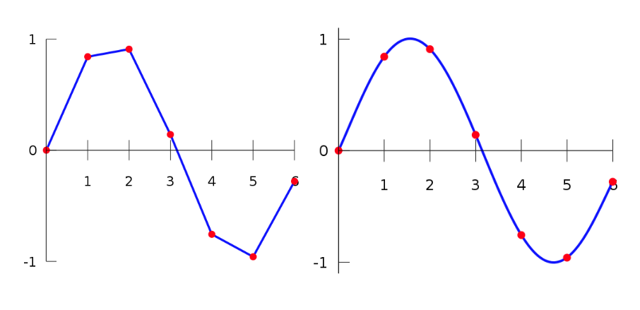
Interpolation can be linear, meaning we construct straight lines between points, or spline, meaning a smooth curve is fitted to provided points. With a small number of points, linear interpolation will yield cusp edges but splines will always be smooth. However, with some point sets, to maintain that smoothness, splines might wander dangerously far away from whichever curve was being fitted in the first place so use that with caution. In most cases, if you have enough points, linear interpolation will be just fine.
Interpolated curves start at parameter $t=0$ which represents the first passed point, and ends at $t=1$ which is coincident with the last point.
See the examples/complex/airfoil.py tutorial for a brief demonstration of curve usage:
def get_curve(z: float) -> cb.SplineInterpolatedCurve:
    """Loads 2D points from a Selig file and
    converts it to 3D by adding a provided z-coordinate."""
    raw_data = np.loadtxt(FILE_NAME, skiprows=1) * CHORD
    z_dimensions = np.ones((len(raw_data),)) * z
    points = np.hstack((raw_data, z_dimensions[:, None]))

    curve = cb.SplineInterpolatedCurve(points)
    curve.rotate(f.deg2rad(-ANGLE_OF_ATTACK), [0, 0, 1])

    return curve

bottom_foil_curve = get_curve(0)
top_foil_curve = get_curve(1)
Discrete Curve
When we plan to use exactly the points we have, without interpolation, a discrete curve is the tool for the job. Its purpose is only to find the closest point. Parameter $t$ is actually an index in point array and discretization will always yield the original points, albeit a shorter list if different bounds are specified.
Using Curves to Create Edges
The above objects are curves but not yet block edges. Fortunately, instead of wrestling with point arrays for spline and polyLine edges, classy_blocks provides a single edge type for all of the above curves: OnCurve. All it needs is a single Curve object. It will then find the closest parameter for start and end point and discretize the curve between so that the desired edge will be created.
loft = Loft(...)
loft.bottom_face.add_edge(0, cb.OnCurve(bottom_foil_curve))
loft.top_face.add_edge(0, cb.OnCurve(top_foil_curve))
The beauty of this is that you don’t need to worry whether that curve starts at the right point or where it ends. Also, you can use the same curve object for many edges. That is also nicely illustrated in the airfoil example where a single curve provides edge data for all blocks around the airfoil.
Options
By default, OnCurve edges will create a spline edge in blockMeshDict unless you specify polyLine manually:
edge = cb.OnCurve(curve, representation="polyLine")
By default, 15 points will be created for an Analytic curve, 10 for both interpolated ones. Discrete curve will not invent new points but simply reuse what you provided to construct it. Make sure there is more than one between your block vertices!
If you want to override this default number, use this parameter:
edge = cb.OnCurve(curve, n_points=5)
Now that you are an expert on curves, let’s use them on a real-life example: the airfoil tutorial.